primary visual cortex = striate cortex = brodmann area 17 = BA17 = visual area 1 = v1 !!!!!
The nervous system is not the simplest of systems, but I guess researchers so far have been dissatisfied with its complexity since they've decided to give the same bit several names! This happens a lot throughout the brain, and even more so if you do cross-species comparison. In the case of the primary visual cortex, the six names in common use are given in the title above. Just as a matter of interest, the striate cortex is the anatomical definition (because it looks stripey), the primary visual cortex is the functional name (because it's the first bit of cortex that visual information reaches), and visual area 1, or V1, are other ways of saying this. Brodmann's area 17, or BA17, are an older way of dividing up the cortex, invented by Korbinian Brodmann.
Anatomically, it's the bit of brain at the very back of your skull. It's also the biggest bit of visual cortex, and a clue to why it is bigger than the other areas can be seen in the model on my Neurons fire & ideas emerge page.
Anatomically, it's the bit of brain at the very back of your skull. It's also the biggest bit of visual cortex, and a clue to why it is bigger than the other areas can be seen in the model on my Neurons fire & ideas emerge page.
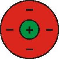
receptive fields prior to v1On the previous page we made a little model of bipolar cells and saw how they were most sensitive to centre surround spots, such as the one on the right.
Still within the retina, there are retinal ganglion cells that also have circular centre-surround receptive field, and then in the thalamus there are the lateral geniculate nuclei, whose cells again have the same kind of receptive fields. It is unlikely that either of these (RGCs and LGN cells) are performing no additional function over the bipolar cells, and there is evidence for certain functions (particularly in the RGCs), but, as far as I can tell, there is not yet a deep understanding of either of these kinds of cells. |
|
Receptive fields in V1
However, as soon as we get to the first visual processing area in the brain, area V1, receptive fields change considerably. While the centre-surround configuration is maintained, the simple spots of the preceding areas are no longer seen. In their place, we find lines of various orientations and lengths. These were named simple cells by Hubel and Wiesel, to contrast them with the complex cells in V1, which have similar receptive fields, but require the line to be moving and respond best to movement in one direction only. Here's the section of Hubel's book where he talks about simple and complex cell receptive fields.
|
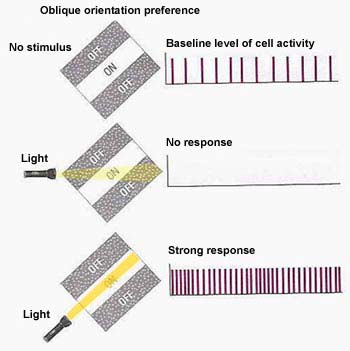
The figure on the left shows the activity of a V1 simple cell with a receptive field oriented diagonally.
It has some baseline level of activity, as shown in the top picture when no light is being shined on its receptive field. If a line of light is shined across its receptive field at an orientation different to that which it is sensitive to, the cell is hyperpolarised (inhibited). If a line of light falls on its receptive field in the orientation it is sensitive to, it becomes strongly depolarised (active). |
How is a linear centre-surround receptive field wired up?
When I first read about this, I was curious as to how the cells sending axons from the retina with their circular centre-surround receptive fields could be wired up to create a linear centre-surround receptive field. Three ways occurred to me: (1) only receiving input from cells which lie on the line, (2) receiving excitatory input both from cells on the line and cells in the surrounding areas, and (3) receiving excitatory input from cells on the line but inhibitory input from cells in the surround. The Hubel book only talks about the first of these, so I decided to do a test to compare them. I'll explain each of the set-ups in a bit more detail.
Note: the bipolar cells that we modelled before determine the circular centre-surround type receptive field, and pass this on to retinal ganglion cells (RGCs) which are the output cells of the retina. RGC axons project to the lateral geniculate nuclei (LGN), which is the final stop before the cortex V1 cells, and also the final place to have the circular configuration. Therefore, when I refer to LGN cells and their messages or receptive fields, I'm talking about the circular centre-surround receptive fields that are sent from the retina.
Note: the bipolar cells that we modelled before determine the circular centre-surround type receptive field, and pass this on to retinal ganglion cells (RGCs) which are the output cells of the retina. RGC axons project to the lateral geniculate nuclei (LGN), which is the final stop before the cortex V1 cells, and also the final place to have the circular configuration. Therefore, when I refer to LGN cells and their messages or receptive fields, I'm talking about the circular centre-surround receptive fields that are sent from the retina.
|
1. Input from the line only.
This is the simplest configuration, requiring the least number of synapses. Only LGN cells whose centres are part of the on section of the line are connected to the V1 cell. The OFF-surround area of the V1 cell is therefore a passive result of the OFF-surrounds of the LGN cells. 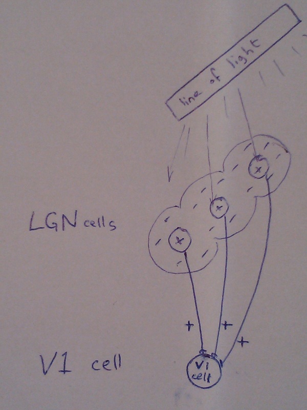
|
2. Excitatory input from cells on the line AND from cells in the surround.
LGN cells with centres in the area surrounding the line are also connected to the V1 cell. Just looking at the picture below, you can see this is more confusing to think about! If a line is shined in the correct place, the cells with centres in the surround should be inhibited, while those with centres on the line are excited. 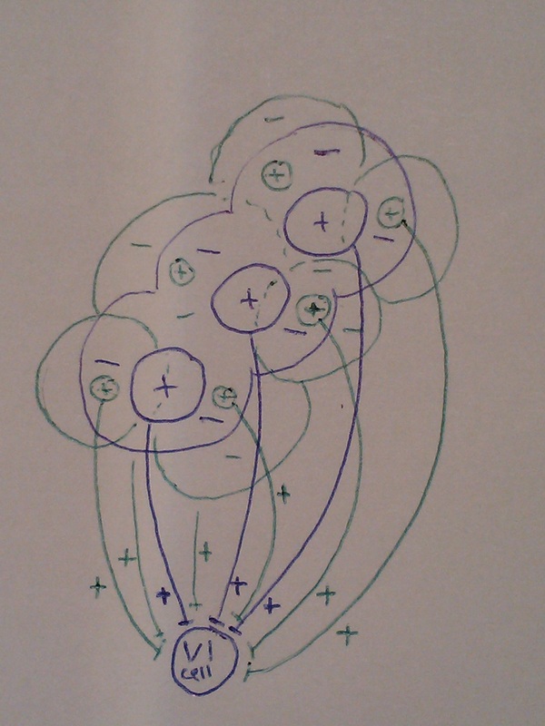
|
3. Excitatory input from cells on the line BUT inhibitory input from cells on in the surround.
Again, LGN cells with centres in areas surrounding the line are also connected to the V1 cell, but this time their inputs are inhibitory, so any light that falls anywhere but on the line will cause the V1 cell to be inhibited. 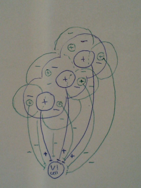
|
Personally and without thinking about it too deeply, I thought (3) was the most convincing because the inhibi. I didn't think (2) would work, and I was dubious about whether (1) would be able to capture the complexity of the behaviour. Of course, if their performance is equal, (1) will be the one favoured by evolution as it is less expensive on resources.
Which one do you think?
Which one do you think?
|
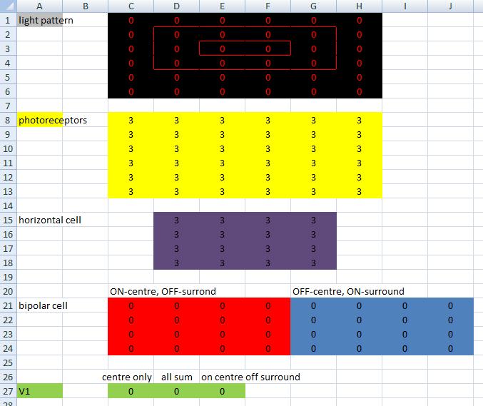
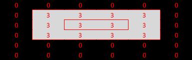
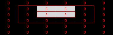
Here's the network I've created to test this. Draw lines in the black light pattern at the top by changing the numbers. 0 = dark, 3 = light (so max value = 3).
There's some info about the other bits of the network in the Excel file, if you're interested. But the important bit for this test is the green bit at the bottom... three V1 cells configured in different ways to suit our three hypotheses. |
|
|
Here's the file -->
|
| ||
the tests
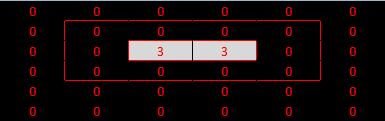
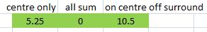
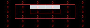
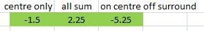
The tests are simply a case of drawing different light patterns and recording the behaviour of the three differently set up V1 neurons to see which performs better. It doesn't matter about the magnitude of the activation, since this can be compensated for by simply strengthening the synapses. However, if the sign of the activation is opposite to what we expect, this is a sign that a given model (wiring) is not appropriate. Below are my tests and results.
|
|
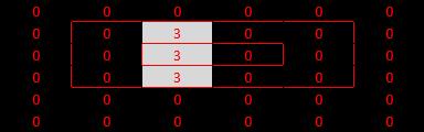
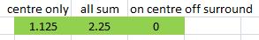
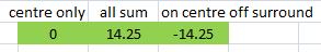
First test: a line of light of exactly the correct orientation and length. This should cause activation in the V1 cell. Model (1) and model (3) behave correctly (remember that magnitude of response is not a concern), whereas model (2) is not active at all - it has failed at the first hurdle! The reason is that each of the cells that have centres in the surrounding area of the line are inhibited due to the light (in their surround), and this inhibition is added to the excitation of the cells with centres on the line. The result is complete equilibrium.
|
|
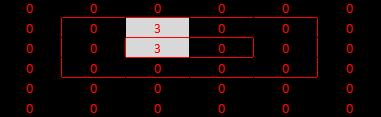
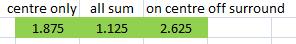
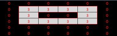
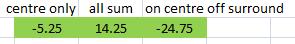
Second test: the same line has been shifted up so that if falls in the surround of the receptive field, rather than the centre. We would expect inhibition of the V1 cell, and that is what we find in models (1) and (3). However, model (2) is misbehaving again. We've shown beyond a shadow of a doubt that model (2) is inappropriate.
|
|
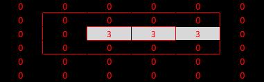
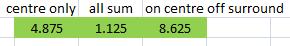
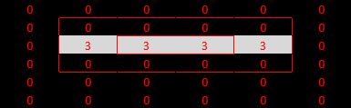
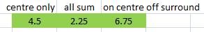
Third test: the line I've used here is a little longer than desired. We'd expect the V1 cell to be active in this case, but perhaps not quite as active as in the previous case. All three models perform well here.
Note: some V1 cells respond best to a line of a certain length, with diminishing activation if the line is either longer or shorter (that's how our model works). However, some V1 cells are completely end-stopped, in that a line which is longer than the receptive field completely inhibits the cell. There are also V1 cells that are not end-stopped at all, so activity increases with increased line length up to the full receptive field length, after which increasing the length of the line makes no difference. See this chapter of Hubel's book for more info.
Note: some V1 cells respond best to a line of a certain length, with diminishing activation if the line is either longer or shorter (that's how our model works). However, some V1 cells are completely end-stopped, in that a line which is longer than the receptive field completely inhibits the cell. There are also V1 cells that are not end-stopped at all, so activity increases with increased line length up to the full receptive field length, after which increasing the length of the line makes no difference. See this chapter of Hubel's book for more info.
|
|
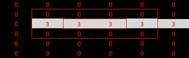
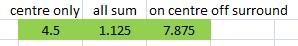
Fourth test: following on from the previous test, we can explore end-stopping a bit more by extending the line in the other direction too. We should see either no change in activation, or decreased activation (since the line is extending beyond the ON-centre). As you can see, the second model is misbehaving again, having increased in activation from the previous test.
The other two models both behave fine, having decreased in activation. We could ask ourself a further question: does the different wiring of the two V1 neurons we've created (models 1 and 3) cause a different kind of end-stopped behaviour. We can see that the activation of model (1) has not decreased as much as that of model (3), in either absolute or relative terms. So it seems that model (3) is more strongly end-stopped than (1). Let's try one more test like this. We can lengthen the line a bit more.
The other two models both behave fine, having decreased in activation. We could ask ourself a further question: does the different wiring of the two V1 neurons we've created (models 1 and 3) cause a different kind of end-stopped behaviour. We can see that the activation of model (1) has not decreased as much as that of model (3), in either absolute or relative terms. So it seems that model (3) is more strongly end-stopped than (1). Let's try one more test like this. We can lengthen the line a bit more.
|
|
Fifth test: Here I've extended the line beyond the receptive field. Just looking at models (1) and (3), I was expecting that the activations would not be affected, and this is the case with model (1), but not with model (3), whose activation has actually increased again. This is strange behaviour. Recalling the previous tests, model (3) was active when presented with a line, then became less active when the line was lengthened, then became more active again when the line was lengthened more. The reason for this is a little hard to understand. Remember that the cells in the surround area are connected to the V1 cell via inhibitory synapses - these cells' surround areas are actually outside what we defined as the receptive field of the V1 cell, and because they are inhibitory surround cells which themselves are connected via an inhibitory synapse, this double negative becomes a positive for the V1 cell. So, by inadvertently extending the receptive field of the neuron, we have created some strange behaviour. It would be easy to tes
|
|
Sixth test: a line of the wrong orientation should lead to no response or to inhibition. The only model that behaves correctly here is model (3), with zero activation.
|
|
Seventh test:
|
|
Eighth test:
|
|
Ninth test:
|

|
